AI algorithm for predicting soil texture from K and Th abundances
This web page provides the algorithim and data used for Maino et al. A Deep Neural Network for predicting soil texture using airborne radiometric data, published in open access by Radiation Physics and Chemistry.
Soil texture, due to its clay, silt and sand contents ternary definition, is a particularly difficult characteristic to model using linear regressions with other soil properties and auxiliary variables.
The most promising results in this field have been recently achieved by Machine Learning methods which are able to derive non-linear, non-site-specific models to predict soil texture.
Here we present and provide a Machine Learning algorithm to predict clay and sand soil contents from Airborne Gamma Ray Spectrometry data of K and Th ground abundances.
The algorithm is divided into two files: the first ('Model_training.py') runs model training on the 500 m x 500 m resolution dataset and saves the obtained models, while the second ('20m_x_20m_predictions.py') loads the previously saved models and makes predictions on the refined 20 m x 20 m dataset.
Since the pretrained models are provided alongside the algorithm, the second part can be run independently of the first.
Model construction and training
We will design our ML algorithm as a pair of parallel Deep Neural Networks (DNNs) composed by 4 hidden layers of 16 nodes each, predicting clay and sand soil contents respectively, each from both K and Th abundances input data. The set of hyperparameters that we’ll choose will be:
| Depth = | 4 |
| Width = | 16 |
| Optimizer = | Adam |
| Loss = | Mean Squared Error |
| Learning rate = | 0.001 |
| Batch size = | 16 |
| Activation function = | ReLU |
and we'll determine the number of epochs by the Early Stopping regularization method. As a first step, we'll also normalize input data in the input layer. The scheme of the DNNs will therefore be:
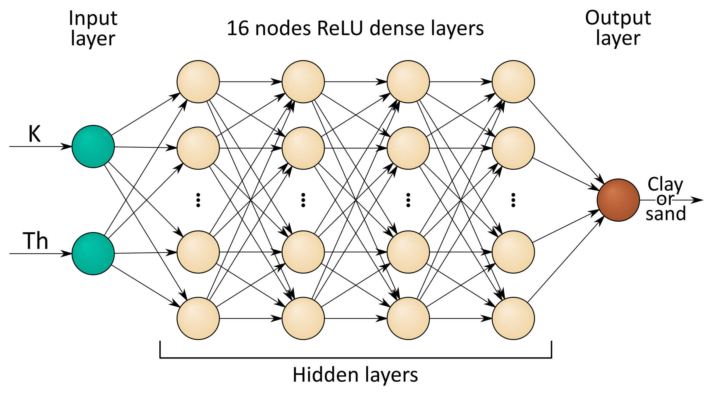
Figure 1: Deep Neural Network model diagram for predicting clay or sand soil contents starting from measured K and Th abundances.
The choice of hyperparameters comes from a series of tests performed on the training dataset. These tests are explained in the original paper
Let's take a look now at the model training Python script.
After importing the necessary libraries, we define the Early Stopping callback to stop training when the loss function value doesn't improve by more than 1 in 5 epochs:
# Earlystopping callback for avoiding unnecessary training epochs
# -> stops training if loss doesn't decrease of at least 1 in 5 epochs
earlystopping = callbacks.EarlyStopping(monitor = 'loss',
                                        min_delta = 1,
                                        patience = 5,
                                        verbose = 0,
                                        mode = 'min',
                                        restore_best_weights = True)
|
Then, we proceed to read the dataset from the file “500x500_dataset.xlsx”. The file is structured in two sheets:
- Train_dataset - contains the 578 training data complete with K and Th abundaces, clay, silt and sand RER soil content measurements, and latitude and longitude;
- Validation_dataset - contains the 72 validation data with the exact same columns of the “Train_dataset” sheet;
- Test_dataset - contains the 73 testing data with the exact same columns of the “Train_dataset” sheet.
We select K and Th abundances from the Train_dataset sheet as training features (same for validation features from the Validation_dataset sheet) and we separate clay and sand soil contents as two different labels, to be used separately by the two parallel DNNs.
# Read training and testing data
Traindata = pd.read_excel('Inputs/500x500_dataset.xlsx', 'Train_dataset', header = [0], engine = 'openpyxl')
Validationdata = pd.read_excel('Inputs/500x500_dataset.xlsx', 'Validation_dataset', header = [0], engine = 'openpyxl')
Testdata = pd.read_excel('Inputs/500x500_dataset.xlsx', 'Test_dataset', header = [0], engine = 'openpyxl')

# Define a Pandas dataframe containing the training data
Train_clay = Traindata['Clay [%]']
Train_sand = Traindata['Sand [%]']
Train_K = Traindata['K [%]']
Train_Th = Traindata['Th [ppm]']

Trainframe = {'K': Train_K, 'Th': Train_Th, 'Clay': Train_clay, 'Sand': Train_sand}
train_dataset = pd.DataFrame(Trainframe)

# Separate the training labels (clay and sand percentages)
train_features = train_dataset.copy()
Sand_train_labels = train_features.pop('Sand')
Clay_train_labels = train_features.pop('Clay')


# Define a Pandas dataframe containing the validation data
Validation_clay = Validationdata['Clay [%]']
Validation_sand = Validationdata['Sand [%]']
Validation_K = Validationdata['K [%]']
Validation_Th = Validationdata['Th [ppm]']

Validationframe = {'K': Validation_K, 'Th': Validation_Th, 'Clay': Validation_clay, 'Sand': Validation_sand}
validation_dataset = pd.DataFrame(Validationframe)

# Separate the validation labels (clay and sand percentages)
validation_features = validation_dataset.copy()
Sand_validation_labels = validation_features.pop('Sand')
Clay_validation_labels = validation_features.pop('Clay')


# Define a Pandas dataframe containing the testing data
Test_clay = Testdata['Clay [%]']
Test_sand = Testdata['Sand [%]']
Test_K = Testdata['K [%]']
Test_Th = Testdata['Th [ppm]']

Testframe = {'K': Test_K, 'Th': Test_Th, 'Clay': Test_clay, 'Sand': Test_sand}
test_dataset = pd.DataFrame(Testframe)

# Separate the testing labels (clay and sand percentages)
test_features = test_dataset.copy()
Sand_test_labels = test_features.pop('Sand')
Clay_test_labels = test_features.pop('Clay')
|
We can now start constructing the algorithms.
Let's start by defining the normalization layer as the standard Keras implementation:
# Define normalization layer (input layer)
normalizer = preprocessing.Normalization(axis = -1)
normalizer.adapt(np.array(train_features))
|
And then construct the clay-predicting DNN structure by adding the input layer (normalization layer) followed by the hidden dense layers with the ReLU activation function and closing it off with a single node output layer:
# Set initial seeds for reproducibility
utils.set_seeds(99999)

# Define sequential model
Clay_model = keras.Sequential()

# Add normalization layer as the input layer
Clay_model.add(normalizer)
# Add 4 hidden layers with 16 nodes each and with the ReLU activation function
for i in range(4):
    Clay_model.add(layers.Dense(16, activation = 'relu'))
# Add single-output layer with 1 node and linear activation function (default)
Clay_model.add(layers.Dense(1))
|
We then compile the model with the desired loss, optimizer and learning rate (lr):
# Compile the model
Clay_model.compile(loss = 'mean_squared_error',                  # Function to be minimized during training
                   optimizer = tf.keras.optimizers.Adam(0.001))  # Algorithm for loss minimization (lr = 0.001)
|
And fit the training features and labels for a maximum of 100 epochs with early stopping, evaluating the performances on the validation dataset while storing the results in a variable called Clay_history:
# Start training
Clay_history = Clay_model.fit(train_features,
                              Clay_train_labels,
                              validation_data = (validation_features, Clay_validation_labels),
                              verbose = 1, epochs = 100,
                              batch_size = 16, callbacks = [earlystopping])
|
Now we can do the same for the sand-predicting DNN, making sure to utilize sand labels instead of clay labels during training:
# Set initial seeds for reproducibility
utils.set_seeds(99999)

# Define sequential model
Sand_model = keras.Sequential()

# Add normalization layer as the input layer
Sand_model.add(normalizer)
# Add 4 hidden layers with 16 nodes each and with the ReLU activation function
for i in range(4):
    Sand_model.add(layers.Dense(16, activation = 'relu'))
# Add single-output layer with 1 node and linear activation function (default)
Sand_model.add(layers.Dense(1))

# Compile the model
Sand_model.compile(loss = 'mean_squared_error',                  # Function to be minimized during training
                   optimizer = tf.keras.optimizers.Adam(0.001))  # Algorithm for loss minimization (lr = 0.001)

# Start training
Sand_history = Sand_model.fit(train_features,
                              Sand_train_labels,
                              validation_data = (validation_features, Sand_validation_labels),
                              verbose = 1, epochs = 100,
                              batch_size = 16, callbacks = [earlystopping])
|
Now that both models have been trained, we can evaluate the accuracy of the models by plotting their loss curves on both the training and validation datasets:
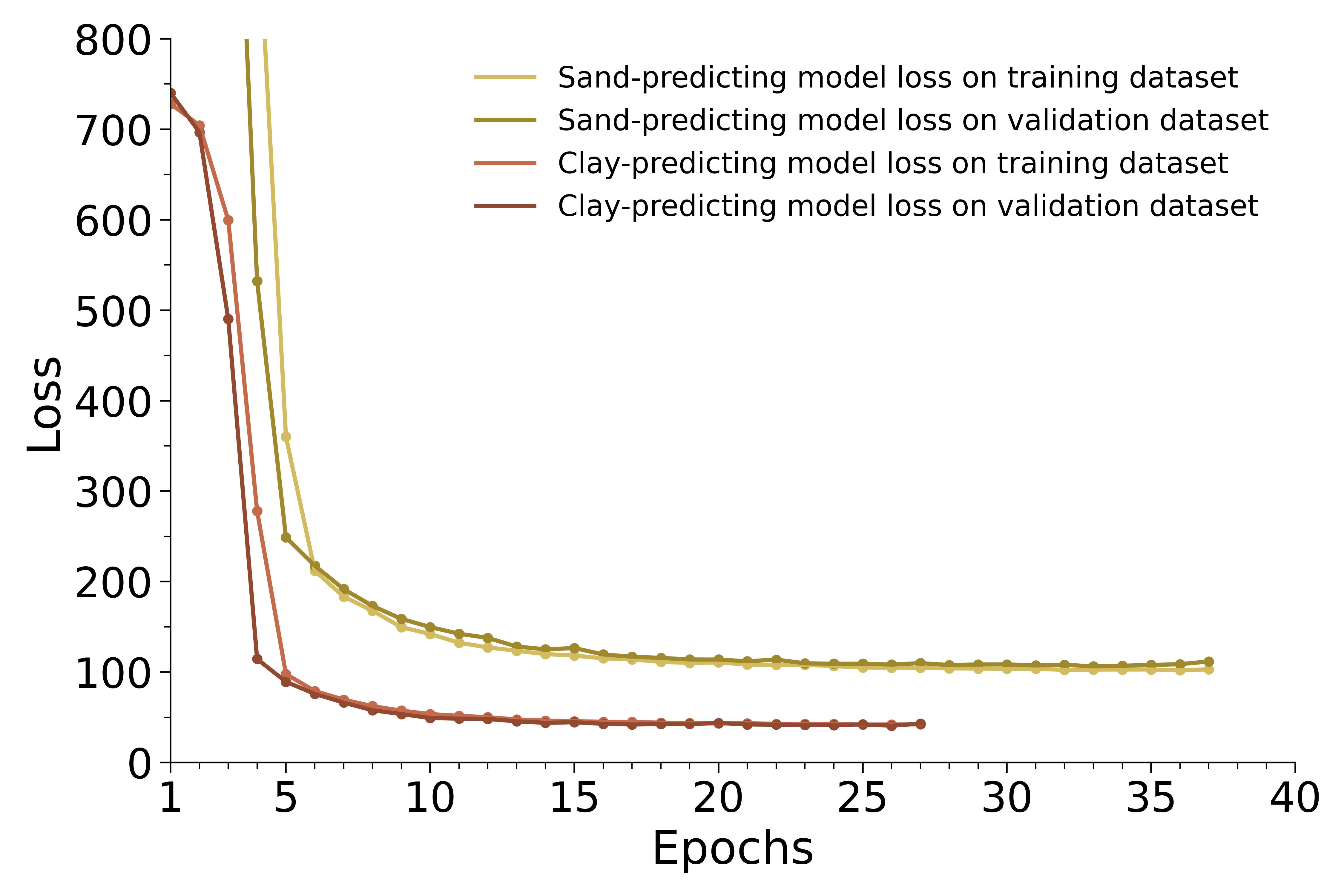
Figure 2: clay-predicting model loss curves on training (light brown) and validation (brown) datasets, together with sand-predicting model loss curves on training (light gold) and validation (gold) datasets.
and predict labels from the testing dataset:
# Predict on test features
Clay_predictions = Clay_model.predict(test_features, batch_size = 16, verbose = 1).flatten()
Sand_predictions = Sand_model.predict(test_features, batch_size = 16, verbose = 1).flatten()
|
If we are satisfied with the results, we can now save the models (both DNN architecture and learned parameters) as Tensorflow readable files in the 'Models' folder:
Clay_model.save('Models/Clay_model', save_format = 'tf')
Sand_model.save('Models/Sand_model', save_format = 'tf')
|
20 m x 20 m resolution predictions
Now that we’ve trained our models, we can apply them to a refined AGRS K and Th abundance map with a resolution of 20 m x 20 m.
After importing the same libraries utilized by the training script, we can load the saved models:
Clay_model = tf.keras.models.load_model('Models/Clay_model')
Sand_model = tf.keras.models.load_model('Models/Sand_model')
|
We can then read the high resolution AGRS data from the file 'K_Th_20x20.xlsx':
Preddata = pd.read_excel('Inputs/K_Th_20x20.xlsb', 'K_Th_20x20', header = [0], engine = 'pyxlsb')

PredLat = Preddata['Latitude']
PredLon = Preddata['Longitude']
PredK = Preddata['K [%]']
PredTh = Preddata['Th [ppm]']

Predframe = {'Latitude': PredLat, 'Longitude': PredLon, 'K': PredK, 'Th': PredTh}
pred_dataset = pd.DataFrame(Predframe)

pred_features = pred_dataset.copy()
disp1 = pred_features.pop('Latitude')
disp2 = pred_features.pop('Longitude')
|
Now that we have both the models and the input data prepared, we can make predictions on the 20 m x 20 m dataset and add the results to the dataframe built during data reading:
Clay_preds = Clay_model.predict(pred_features, batch_size = 16, verbose = 1).flatten()
Sand_preds = Sand_model.predict(pred_features, batch_size = 16, verbose = 1).flatten()

pred_dataset['Clay'] = Clay_preds
pred_dataset['Sand'] = Sand_preds
|
Let's now visualize our results by plotting the clay and sand soil contents predictions into the USDA soil textural triangle:
# Create list of matching clay and sand predictions
data = []
for num in range(len(pred_dataset['Clay'])):
    data.append([pred_dataset['Clay'][num], pred_dataset['Sand'][num]])

# Turn list into array
datarray = np.asarray(data)

# Draw the USDA textural triangle
texture.draw_triangle(datarray, save = True, save_path = 'Outputs/20x20_predictions_triangle')
|
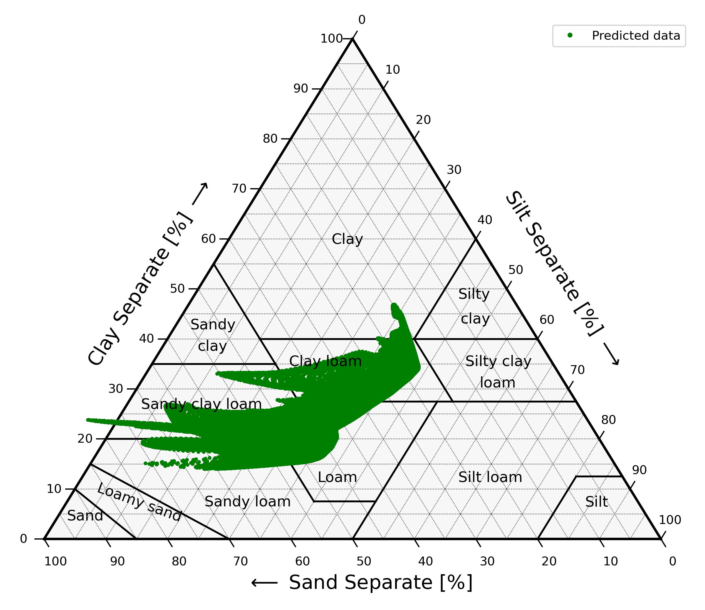
Figure 3: USDA textural triangle containing the predicted textural compositions. Silt is inferred as 100 % - clay content - sand content.
As we can see, the models produce 59 predictions outside of the textural triangle. That can happen because no limit was imposed on the predicted clay and sand contents, so in this case the sum of the clay and sand components exceeds the 100 % limit.
When assigning a textural class to these compositions, we fix this by rescaling the clay and sand sum to 100 % (implemented in the 'soiltexturalclass' function inside the 'texture.py' file).
As a final step, we save the models' predictions and the corresponding textural classes in an Excel file:
# Create Excel file
workbook = xlsxwriter.Workbook('Outputs/Texture_map_20x20.xlsx')
worksheet = workbook.add_worksheet('Texture_map_20x20')

# Write column headers
worksheet.write(0, 0, 'Latitude')
worksheet.write(0, 1, 'Longitude')
worksheet.write(0, 2, 'K [%]')
worksheet.write(0, 3, 'Th [ppm]')
worksheet.write(0, 4, 'Clay [%]')
worksheet.write(0, 5, 'Sand [%]')
worksheet.write(0, 6, 'Textural class')

# Write data
for i in range(Clay_preds.shape[0]):

    try:
        worksheet.write(i + 1, 0, pred_dataset['Latitude'][i])
        worksheet.write(i + 1, 1, pred_dataset['Longitude'][i])
        worksheet.write(i + 1, 2, pred_dataset['K [%]'][i])
        worksheet.write(i + 1, 3, pred_dataset['Th [ppm]'][i])
        worksheet.write(i + 1, 4, pred_dataset['Clay [%]'][i])
        worksheet.write(i + 1, 5, pred_dataset['Sand [%]'][i])
        worksheet.write(i + 1, 6, texture.soiltexturalclass(Sand_preds[i], Clay_preds[i]))
    except:
        pass

workbook.close()
|
The dataset, models, Python scripts and Anaconda environment files can be downloaded at this link: