Charge Reconstruction Algorithm
This web page provides the algorithim published in Grassi et al. Charge reconstruction in large-area photomultipliers, 2018 JINST 13 P02008, arXiv:1801.08690.
The prevalent trend to adopt large area PhotoMultiplier Tubes (PMT), typically with a diameter of 20 inch, has to take into account the non-linear reconstruction of the deposited charge, when a single PMT collects an enough amount of electromagnetic energy to produce more than a single PhotoElectron (PE). This pile up effect is accentuated in the large detector, where the size is comparable to the LS attenuation length. The large acceptance of PMT threatens the time reconstruction of the event and hence of fiducial volume, which is often mandatory to reject background from natural radioactivity. Such fiducialisation relies on the capability to precisely reconstruct the event vertex position, which in turns demands a precise time information.
In a standard 20 inch PMT, for an event of reactor antineutrino in some tens kton detector, more than 50 % of the total charge is collected by more than 1 PE. Although an high frequency sampling of the PMT output waveform provided by Flash Analog-to-Digital Converters (FADCs) improves the calorimetric performance of the detector, an accurate analysis of the digital signal is mandatory for an unbiased reconstruction of input charge and of the photon time of arrival.
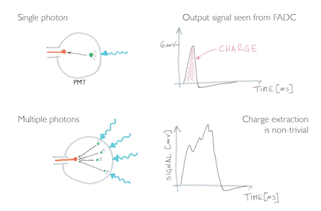
Figure 1: Sketch illustrating of the bias on charge recontruction due to multi-hit on a PMT.
The main purpose of the presented algorithm is to reduce the bias on the reconstructed charge due to the previously described hardware effects.
The algorithm is structured in three parts: the first is used to analyze the input file with Digital Signal Processing technique as filtering and deconvolution (Deconvolution Algorithm - DA) and reconstruct the charge (Integration Algorithm - IA), the second is used to generate the SPE shape as input for the first algorithm, while the third is used to generate events in order to validate the first one (Event Building).
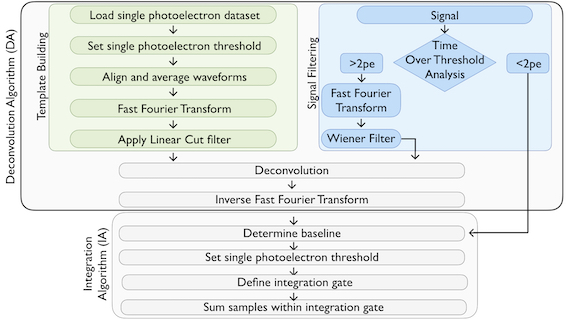
Figure 2: schematic diagram of the charge reconstruction algorithm. The SPE template in the time domain is computed by averaging 104 SPE waveforms that simulate an LED-based calibration dataset. A Fast Fourier Transform (FFT) is applied to both the SPE template and the pmt waveform to be reconstructed. The latter is processed using the Wiener Filter to minimize the noise and suppress the overshoot. The SPEs template in the frequency domain is then used as a benchmark pattern to deconvolve the filtered waveform in the frequency domain. We eventually process the deconvolved waveform with an Inverse FFT, so that the waveform in the time domain could be integrated to compute the pmt output charge.
Filter and Deconvolution Algorithm
Input File Structure
We need three different input file an SPE template, a Noise waveform sample and a ROOT file containing the waveforms to be processed. The files has to be placed in a folder under the following path:
./data/
The first file has to be a text file named SPE_shape.txt with the following structure
| # SPE_charge = | 0.964687 |
| # i_max_SPE = | 250 |
| # th_SPE = | 6 |
| # flex_point = | 6 |
| # nSamples = | 1000 |
| # time | #value |
| 0 | 0.891323 |
| 1 | 1.20741 |
| . | . |
| . | . |
The second has to be a text file named Noise.txt with the following structure
| # time | #value |
| 0 | 1 |
| 1 | 0 |
| 2 | 3 |
| . | . |
| . | . |
The third is a *.root files containing a ROOT Tree named “waveforms_unblinded” with the following structure for entries:
| Variable Name | Variable Type | Description |
|---|---|---|
| nHit | Integer | Number of pulse in the events |
| time [nHit] | Array of Float | Array of the hit time of each pulse |
| charge [nHit] | Array of Float | Array of the charge Produced by each pulse |
| nSample | Integer | Number of the sampling point of the waveform |
| waveform [nSample] | Array of Integer | Waveform to be analysed |
Table 1: Structure of the tree in the *.root input files
It is possible to generate SPE_shape.txt and Noise.txt with the algorithm presenteted in the Calibration Section.
An example of functional data folder can be downloaded here.
Input Parameter for the Charge Reconstruction Algorithm
To work properly the macro need a config file situated in ./conf/config_CRA.txt with the following structure
| # num_event = 10000 |
| # num_max_hit = 16 |
| # fc = 120 |
| # SPE_filt = l |
| # Sign_filt = wd |
| # bin_area = 6 |
| # time_ov_threshold = 4 |
Where:
- # num_event: is the number of events to be analyzed
- # num_max_hit: is the maximum number of hits (used for build the graph)
- # SPE_filt: is the Digital Signal Processing (DSP) technique use for the SPE shape construction
- # Sign_filt:is the Digital Signal Processing (DSP) technique use for the waveform analysis
- # fc: is the frequency cut
- # bin_area: is the lenght of the Region of Integration ROI
- # time_ov_threshold: is used to define the minimum lenght (min lenght = time_ov_threshold * SPE_length) of the waveform over the threshold in order to discriminate the waveforms where to adopt the filter
The DSP tecnique that are implemented are listed below
| Filter Type | Command |
|---|---|
| Windowed Sync Filter | s |
| Average Filter | a |
| Chebychev Filter | c |
| Wiener Filter optimized for each event | w |
| Wiener Filter Built from the SPE shape | k |
| Deconvolution | d |
Table 2: List of the Digital Signal Processing techniques implemented in the code
To use the desired technique just input, when request, the correspondent letter of the filter you want to use (i.e. for the Windowed Sync Filter use s). In case you want to use more than one process input both the letters following your desired sequence (i.e. if you want to use Optimized Winer Filter and Deconvolution input wd).
After starting the macro it will ask for folder where to find the *.ROOT input file.
Output of the DA (Deconvolution Algorithm)
The output of the DA are the waveform to be processed by the IA (Integration Algorithm).
See example
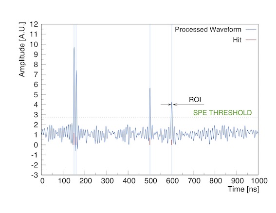
Figure 3: waveform arising from filtering and deconvolving a waveform. True hits are shown for reference in red. The charge of each pe is reconstructed by integrating the the bins falling within a Region Of Interest (shaded areas) defined starting from the time at which the waveform crosses a trigger threshold (dashed line). The threshold is set to be 30% of the amplitude of a SPE pulse.
Output of the DA and of the IA
The output of the algorithm is a plot of the Reconstructed Charge vs Real Charge with the parameter of the linear correlation given in the form of the angular coefficient m, the y-intercept q and the value of the Pearson’s coefficient. See Fig.3
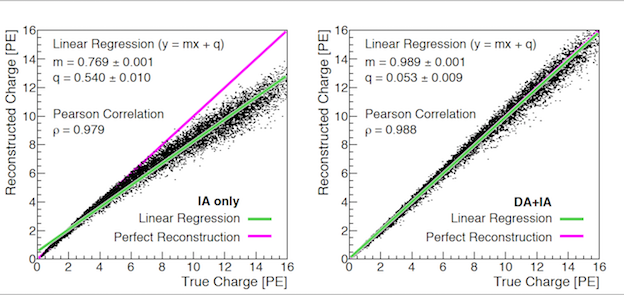
Figure 4: reconstructed charge versus true charge for 104 pmt waveforms. The reconstructed charge is computed using the IA alone (left) and DA+IA (right). In both panels the green line is the result of a linear regression performed on the 104 data points.
Calibration Algorithm
Input Calibration Algorithm
The input of the Calibration Algorithm is a *.root files containing a ROOT Tree named “waveforms_unblinded” with the following structure for entries:
| Variable Name | Variable Type | Description |
|---|---|---|
| nHit | Integer | Number of pulse in the events |
| time [nHit] | Array of Float | Array of the hit time of each pulse |
| charge [nHit] | Array of Float | Array of the charge Produced by each pulse |
| nSample | Integer | Number of the sampling point of the waveform |
| waveform [nSample] | Array of Integer | Waveform to be analysed |
Table 1: Structure of the tree in the *.root input files
In the ROOT file are stored waveform samples coming form an LED calibration of the PMT
To work properly the macro need a config file situated in ./conf/config_cal.txt with the following structure
| # nSamples = 1000 |
| # nSPE = 16 |
Where:
- # nSamples: is the number of sampling point of each waveform
- # nSPE: is the maximum number of SPE waveform to be used for the building of the template
Output of Calibration Calibration
The algorithm will give two different outputs stored in the folder ./data/data_folder
1)The Noise sample in the file Noise.txt
2)The SPE template stored in SPE_template.txt
both with the structure showed in the Reconstruction Section
Event Building Algorithm
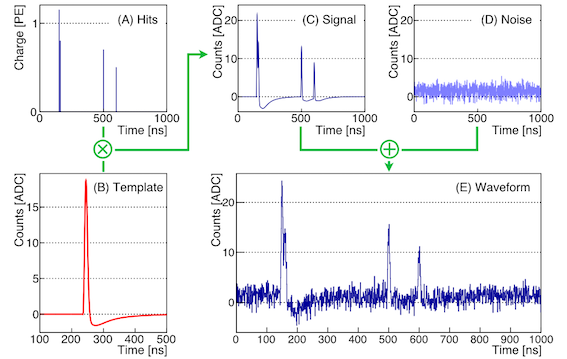
Figure 5: building blocks of the waveform simulation. Panel A shows the hit generation, where for each detected PE a random charge value is generated. Panel B shows the analytical shape of a Single PE (SPE)template. Panel C is the result of the convolution between the SPE template and the hits. Panel D contains the PMT noise simulation. Panel E shows the final PMT waveform resulting from the sum of the signal and of the noise components.
In order to validate the FDA and CRA is given an algorithm used to produce the input files to be processed by the analysis algorithm.
Input of the Synthetic Waveform Production Algorithm
The SPE spectrum is parametrized by the equation [2.1] explicated in the paper
The main parameters are:
| Parameter | Adopted values | Variable in the code |
|---|---|---|
| q0 = SPE calibrated gain | 1 PE | q0 |
| qp = Pedestal cutoff | 0.3 PE | qp |
| σ = SPE resolution | 0.3 PE | sigmaq |
| ω = Tail-to-Gaussian ratio | 0.2 | w |
| τ = Tail decay constant | 0.5 PE | tq |
Table 4: List of the parameters used to simulate the SPE spectrum
These values can be changed in the EventsCreator.cc file.
The SPE waveform is simulated by a peak and an overshoot as ilustarted by the equations [2.2-2.5] in the paper.
The main parameters used in the simulation are enlisted in the following table
| Parameter | Adopted values | Variable in the code |
|---|---|---|
| U0 | 20 ADC | U |
| σ0 | 0.15 | sigma |
| τ0 | 30 ns | tau |
Table 5: List of the parameters used to simulate the peak of SPE shape
| Parameter | Adopted values | Variable in the code |
|---|---|---|
| U1 | -1.2 ADC | U1_os |
| σ1 | 55 ns | sigma1_os |
| t1 | -4 ns | t1_os |
| Parameter | Adopted values | Variable in the code |
|---|---|---|
| U2 | -2.8 ADC | U2_os |
| t2 | 80 ns | tau_2_os |
Table 6-7: List of the parameters used to simulate the overshoot of SPE shape
The noise is modelled with a Gaussian noise parametrized by
| Parameter | Adopted values | Variable in the code |
|---|---|---|
| μ = the average of the Gaussian Distribution | 1.5 ADC | mu_noise_wave |
| σ = the standard deviation of the Gaussian Distribution | 1 ADC | sigma_noise_wave |
| nFF = Number of components | 5 | n |
| fFF = fixed frequencies | [1, 480] MHz | f |
| A = the mean amplitude of the Noise | A = [0.1, 0.3] ADC | A |
Table 8: List of the parameters used to simulate the noise
We simulate also non-Gaussian noise due to the external and internal electronics by adding specific frequencies to the Gaussian Noise spectrum parametrized as follows
1) n_peak is the number of the specific frequencies
2) They will have, by default, a frequency in the range [50 MHz; 150MHz] and each one will produce a noise with an height between [0 ADC, 1 ADC].
All the parameter can be varied modifying the config file situated in ./conf/config_evt.txt
| # num_event = 10000 |
| # num_max_hit = 16 |
| # n_peak = 20 |
| # nSamples = 1000 |
| # U = 20 |
| # tau = 30 |
| # sigma = 0.15 |
| # U1_os = -1.2 |
| # t1_os = -4 |
| # sigma1_os = 55 |
| # U2_os = -2.8 |
| # tau_2_os = 80 |
| # t2_os_0 = 50 |
| # t2_os_1 = 10 |
| # deltax = 215 |
| # mu_noise = 1.5 |
| # sigma_noise = 1 |
Where:
- # num_event: is the number of events to be analyzed
- # num_max_hit: is he maximum number of hits (used for build the graph)
- # nSamples: is the number of sampling point of each waveform
Output of the Synthetic Waveform Production Algorithm
The Output of the Synthetic Waveform Production Algorithm are two *.root files called LED_unblinded.root and physics_unblinded.root containing the tree to be analysed by the Calibration Algorithm and by the Charge Reconstruction Algorithm respectively.
The algorithms can be downloaded at this link.