Iterative Harmonic Correction Framework (IHCF) for microgravity base-station drift

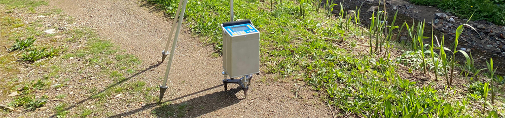
This web page provides the Python code associated with Petrone et al., Iterative harmonic drift correction for the Scintrex CG-5 gravimeter, submitted to Geophysics.

Microgravity surveys with portable relative gravimeters target anomalies of a few tens of µGal, an amplitude comparable to the bias introduced by unmodeled instrumental drift. The standard practice of repeated base-station occupations followed by linear or low-order polynomial detrending leaves a residual variability that, in the nine datasets analyzed in the paper (eight field campaigns and one 21-day laboratory benchmark, acquired with a Scintrex CG-5 between 2021 and 2025), exceeds the geological signal by up to two orders of magnitude. The Iterative Harmonic Correction Framework (IHCF) addresses this limitation with a single-instrument, operator-independent procedure that models the systematic component of base-station drift as a sum of deterministic harmonic terms identified directly from the data, without prescribing a functional form a priori.

The implementation is contained in a single Python script that processes a folder of CG-5 CSV exports in batch and, for each site, produces (i) a corrected residual time series, (ii) a tabulation of the accepted harmonic components with covariance-derived uncertainties, (iii) a per-site three-panel diagnostic figure, and (iv) panel summaries comparing all sites. The pipeline is reproducible by personnel without specialized gravimetric training.

Configuration

All thresholds, period bands and grid sizes are exposed as module-level constants at the top of the script. The default values reproduce the paper results.

# Memory-jump detection
JUMP_THRESHOLD = 5.0      # mGal
MIN_GAP_POINTS = 3

# Period bands explored at each iteration
LONG_MIN_DAYS  = 4.0
LONG_MAX_DAYS  = 200.0
SHORT_MIN_DAYS = 0.5      # 12 h
SHORT_MAX_DAYS = 4.0      # 96 h

# Minimum separation between accepted periods within the same band
MIN_SEP_LONG_DAYS    = 5.0
MIN_SEP_SHORT_HOURS  = 4.0

# Grid resolution and safety bound on the number of components
GRID_LONG       = 5000
GRID_SHORT      = 5000
MAX_COMPONENTS  = 20

# Stopping criteria
# 1) global criterion: chi2_red <= 1 + sqrt(2/nu)
# 2) incremental criterion: Delta chi2 > 3 ln N + DELTA_EXTRA
DELTA_EXTRA = 6.0

The constant DELTA_EXTRA = 6 corresponds to the threshold of strong evidence on the Kass and Raftery (1995) scale for Bayes factors, and ensures that components are accepted only when the data provide solid statistical support. The factor 3 ln N is the standard Bayesian information criterion (BIC) penalty for the three additional parameters introduced by each new harmonic (sine and cosine coefficients plus the period selected by the grid search).

Input parsing

Each base-station record is a CSV exported from the CG-5 with the firmware Earth-tide correction enabled. The loader requires three columns — a datetime field, the firmware-corrected gravity value and the per-sample standard deviation — and discards samples whose declared uncertainty exceeds the configurable threshold.

def load_dataset(filepath):
    df = pd.read_csv(filepath, sep=';', encoding='utf-8-sig')
    df.columns = [c.strip().upper() for c in df.columns]

    # robust column lookup
    time_col = next((c for c in df.columns if "DATETIME" in c), None)
    grav_col = next((c for c in df.columns if "GRAV_CORRTIDE" in c), None)
    sd_col   = next((c for c in df.columns if c == "SD"), None)

    dt = pd.to_datetime(df[time_col], dayfirst=True, errors="coerce")
    out = pd.DataFrame({
        "DATETIME": dt,
        "g":        pd.to_numeric(df[grav_col], errors="coerce"),
        "sigma":    pd.to_numeric(df[sd_col],   errors="coerce"),
    }).dropna(subset=["DATETIME", "g", "sigma"]).sort_values("DATETIME").reset_index(drop=True)

    # keep only records with declared sigma below the trust threshold
    out = out[out["sigma"] < 10.07].reset_index(drop=True)
    out["source_file"] = os.path.basename(filepath)
    return out

Memory-jump correction

Sustained operation of the CG-5 periodically exhausts the on-board memory: each reset introduces a discontinuity in the recorded gravity series whose amplitude can reach hundreds of mGal and which is not captured by the firmware drift model. The memory-jump correction detects events where the absolute difference between consecutive base-station readings exceeds JUMP_THRESHOLD (5 mGal by default, several orders of magnitude above the instrumental repeatability and below the typical post-reset offset). For each detected reset, the offset Δg between the last reading before and the first reading after is applied as a constant correction to all subsequent values, restoring continuity across memory-bounded segments and yielding a single continuous reference sequence.

def correct_memory_reset(g, threshold=JUMP_THRESHOLD, min_gap=MIN_GAP_POINTS):
    g = np.asarray(g, float)
    n = len(g)
    if n < 2:
        return g.copy(), np.array([], dtype=int), np.array([], dtype=float)

    # detect candidate jumps and merge events too close in time
    diffs = np.diff(g)
    jumps = np.where(np.abs(diffs) > threshold)[0] + 1
    if jumps.size:
        compact = [jumps[0]]
        for j in jumps[1:]:
            if j - compact[-1] > min_gap:
                compact.append(j)
        jumps = np.array(compact, dtype=int)

    # apply Delta_g segment by segment
    bounds = np.r_[0], jumps, n]
    g_corr = g.copy()
    deltas = []
    for si in range(1, len(bounds) - 1):
        e_prev = bounds[si]
        s_cur  = bounds[si]
        e_cur  = bounds[si + 1]
        delta = g_corr[e_prev - 1] - g_corr[s_cur]
        g_corr[s_cur:e_cur] += delta
        deltas.append(delta)
    return g_corr, jumps, np.array(deltas, float)

Single-period weighted fit

The building block of the iterative search is a heteroscedastic weighted least squares fit at a fixed period T. The model is the linear sine–cosine form

y(t) = a sin(ωt) + b cos(ωt) + c,     ω = 2π / T

with weights w_i = 1/σ_i². Component amplitude and phase follow as A = √(a² + b²) and φ = atan2(b, a); the full covariance matrix is propagated to obtain σ_A and σ_φ.

def fit_period_linear(t_days, y, sigma, T_days):
    omega = 2.0 * np.pi / T_days
    X = np.column_stack([
        np.sin(omega * t_days),
        np.cos(omega * t_days),
        np.ones_like(t_days)
    ])
    w   = 1.0 / sigma**2
    WX  = X * w[:, None]
    XtWX = X.T @ WX
    XtWy = X.T @ (w * y)
    beta = np.linalg.solve(XtWX, XtWy)
    cov  = np.linalg.inv(XtWX)
    yhat = X @ beta
    resid = y - yhat
    chi2 = np.sum((resid / sigma) ** 2)
    a, b, c = beta
    amp   = np.sqrt(a*a + b*b)
    phase = np.arctan2(b, a)
    return {"T_days": T_days, "chi2": chi2, "yhat": yhat,
            "amp": amp, "phase": phase, "offset": c,
            "beta": beta, "cov": cov, "resid": resid}

The wrapper search_band applies fit_period_linear to every period of the long or short grid, skipping candidates that violate the minimum-separation constraint with respect to already accepted periods, and returns the candidate that minimises χ².

Iterative competitive search

The model is built iteratively. The initial state is the weighted mean of the memory-corrected series, serving as a single-parameter offset. At each iteration, residuals are computed from the current cumulative model, and search_band is applied independently to the short and to the long band. The two band champions then compete, and the candidate producing the larger reduction of χ² is retained as the proposed component for that iteration. This competitive structure permits the algorithm to alternate between fast and slow timescales as the data require, rather than exhausting one band before exploring the other.

Two stopping criteria govern the loop. The global stopping criterion compares the reduced chi-square of the current model to its expected statistical fluctuation under the null hypothesis of Gaussian residuals,

χ²_red ≤ 1 + √(2 / ⟨χ²⟩)

and is satisfied when residuals are statistically indistinguishable from the noise floor. The incremental acceptance test admits the proposed component only if

Δχ² > 3 ln N + 6

where the term 3 ln N is the standard BIC penalty for the three additional parameters (a, b, T) and the constant 6 is the Kass–Raftery threshold of strong evidence. The iteration terminates when neither band champion satisfies the incremental test, or when the global criterion is met after an accepted component, or when the safety bound MAX_COMPONENTS = 20 is reached.

p_current = 1     # initial model: weighted mean only
delta_threshold = 3.0 * np.log(N) + DELTA_EXTRA

for k in range(1, MAX_COMPONENTS + 1):

    # 1) global criterion on the current model
    prev_metrics = compute_metrics(resid_current, sigma_ug, p_total=p_current)
    if prev_metrics["chi2_red"] <= prev_metrics["abs_stop"]:
        break

    # 2) competitive search: short band vs long band
    candidates = []
    for band_name in ["long", "short"]:
        best = search_band(t_days, resid_current, sigma_ug, band_name, accepted_periods)
        if best is None:
            continue
        trial_model = model_current + best["yhat"]
        trial_resid = g_corr_ug - trial_model
        met = compute_metrics(trial_resid, sigma_ug, p_total=p_current + 3)
        candidates.append({"band": band_name, "best": best,
                           "trial_model": trial_model, "trial_resid": trial_resid,
                           "metrics": met,
                           "delta_chi2": prev_metrics["chi2"] - met["chi2"]})

    if not candidates:
        break

    winner = min(candidates, key=lambda x: x["metrics"]["chi2"])

    # 3) incremental acceptance test (Eq. 3 of the paper)
    if winner["delta_chi2"] <= delta_threshold:
        break

    # 4) accept the new component and re-check the global criterion
    model_current = winner["trial_model"]
    resid_current = winner["trial_resid"]
    p_current += 3
    accepted_periods.append((winner["best"]["T_days"], winner["band"]))
    new_metrics = compute_metrics(resid_current, sigma_ug, p_total=p_current)
    if new_metrics["chi2_red"] <= new_metrics["abs_stop"]:
        break

Global weighted least-squares refit

The harmonics identified iteratively at fixed candidate periods are not orthogonal in general, and a sequential fit introduces a small bias on the estimated coefficients. Once the iterative loop has selected the set of accepted periods {T_i}, a final global weighted least-squares adjustment refits all sine–cosine coefficients simultaneously with the periods held fixed. This step removes the sequential-fitting bias and provides covariance-derived uncertainties on amplitudes and phases.

def global_refit_fixed_periods(t_days, y, sigma, periods_days):
    cols = [np.ones_like(t_days)]
    for T in periods_days:
        omega = 2.0 * np.pi / T
        cols.append(np.sin(omega * t_days))
        cols.append(np.cos(omega * t_days))
    X = np.column_stack(cols)
    w = 1.0 / sigma**2
    beta = np.linalg.solve(X.T @ (X * w[:, None]), X.T @ (w * y))
    cov  = np.linalg.inv(X.T @ (X * w[:, None]))
    yhat = X @ beta
    resid = y - yhat
    # amplitude, phase and covariance-derived uncertainties for each component
    components = []
    for j, T in enumerate(periods_days):
        a = beta[1 + 2*j]
        b = beta[2 + 2*j]
        components.append({
            "T_days":   T,
            "amp_ug":   np.sqrt(a*a + b*b),
            "phase_rad": np.arctan2(b, a),
            # sigma_a, sigma_b, sigma_amp, sigma_phase from covariance propagation
        })
    return {"yhat": yhat, "resid": resid,
            "offset_ug": beta[0], "components": components}

Outputs and diagnostics

For each site processed by process_site, the script produces a three-panel summary figure with the gravity series and global IHCF fit, the residual distribution with the best-fit Gaussian and the residual time series with the ±σ band:

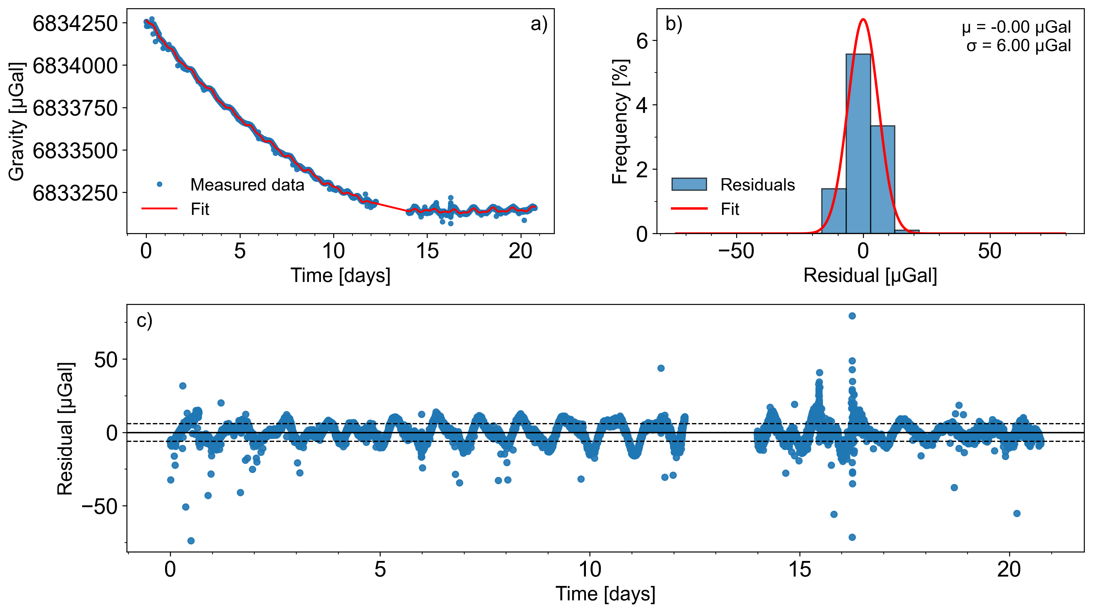
Single-site three-panel diagnostic figure. (a) memory-jump aligned and firmware-tide corrected gravity series with the global IHCF fit; (b) residual histogram with the best-fit Gaussian and (μ, σ) annotations; (c) residual time series with the ±σ band.

At the batch level (main), the script also exports three CSV tables and four panel figures comparing all sites:

Applicability beyond the CG-5

The implementation is not bound to CG-5-specific features: the algorithm operates on any sequence of timestamped readings provided with per-sample uncertainty, and is therefore applicable to other relative gravimeters that supply such input. The only instrument-specific block is load_dataset, which can be replaced by any reader that returns a dataframe with the three required columns (DATETIME, g, sigma); the rest of the pipeline is instrument-agnostic.

Download

The Python script will be made publicly available through this website upon acceptance and publication of the manuscript.