Filter and Deconvolution Algorithm
Input File Structure
We need three different input file an SPE template, a Noise waveform sample and a ROOT file containing the waveforms to be processed. The files has to be placed in a folder under the following path:
./data/
The first file has to be a text file named SPE_shape.txt with the following structure
| # SPE_charge = | 0.964687 |
| # i_max_SPE = | 250 |
| # th_SPE = | 6 |
| # flex_point = | 6 |
| # nSamples = | 1000 |
| # time | #value |
| 0 | 0.891323 |
| 1 | 1.20741 |
| . | . |
| . | . |
The second has to be a text file named Noise.txt with the following structure
| # time | #value |
| 0 | 1 |
| 1 | 0 |
| 2 | 3 |
| . | . |
| . | . |
The third is a *.root files containing a ROOT Tree named “waveforms_unblinded” with the following structure for entries:
| Variable Name | Variable Type | Description |
|---|---|---|
| nHit | Integer | Number of pulse in the events |
| time [nHit] | Array of Float | Array of the hit time of each pulse |
| charge [nHit] | Array of Float | Array of the charge Produced by each pulse |
| nSample | Integer | Number of the sampling point of the waveform |
| waveform [nSample] | Array of Integer | Waveform to be analysed |
Table 1: Structure of the tree in the *.root input files
It is possible to generate SPE_shape.txt and Noise.txt with the algorithm presenteted in the Calibration Section
Input Parameter for the Charge Reconstruction Algorithm
To work properly the macro need a config file situated in ./conf/config_CRA.txt with the following structure
| # num_event = 10000 |
| # num_max_hit = 16 |
| # fc = 120 |
| # SPE_filt = l |
| # Sign_filt = wd |
| # bin_area = 6 |
| # time_ov_threshold = 4 |
Where:
| - # num_event: is the number of events to be analyzed |
| - # num_max_hit: is the maximum number of hits (used for build the graph) |
| - # SPE_filt: is the Digital Signal Processing (DSP) technique use for the sPE shape construction |
| - # Sign_filt:is the Digital Signal Processing (DSP) technique use for the waveform analysis |
| - # fc: is the frequency cut |
| - # bin_area: is the lenght of the Region of Integration ROI |
| - # time_ov_threshold: is used to define the minimum lenght (min lenght = time_ov_threshold * SPE_length) of the waveform over the threshold in order to discriminate the waveforms where to adopt the filter |
The DSP tecnique that are implemented are listed below
| Filter Type | Command |
|---|---|
| Windowed Sync Filter | s |
| Average Filter | a |
| Chebychev Filter | c |
| Wiener Filter optimized for each event | w |
| Wiener Filter Built from the sPE shape | k |
| Deconvolution | d |
Table 2: List of the Digital Signal Processing techniques implemented in the code
To use the desired technique just input, when request, the correspondent letter of the filter you want to use (i.e. for the Windowed Sync Filter use s). In case you want to use more than one process input both the letters following your desired sequence (i.e. if you want to use Optimized Winer Filter and Deconvolution input wd).
After starting the macro it will ask for folder where to find the *.ROOT input file.
Output of the DA (Deconvolution Algorithm)
The output of the DA are the waveform to be processed by the IA (Integration Algorithm).
See example
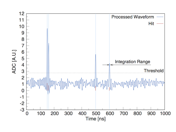
Figure 3: DA output after the use of an optimized Wiener filter and deconvolution
Output of the DA and of the IA
The output of the algorithm is a plot of the Reconstructed Charge vs Real Charge with the parameter of the linear correlation given in the form of the angular coefficient m, the y-intercept q and the value of the Pearson’s coefficient. See Fig.3
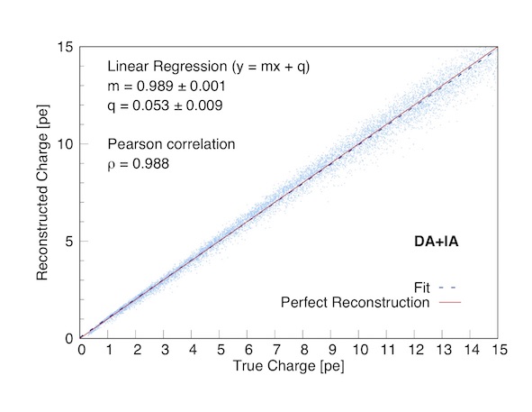
Figure 4: Plot of the reconstructed charges versus real charges for 104 synthetic waveforms. Individual real charge values are determined on the base of the hit distribution generating each synthetic waveform. The reconstructed charge values plotted are obtained with the application of the filtering plus deconvolving algorithm. The blue line corresponds to the best fit linear function interpolating the 104 data points.