Automatic Alert Mail

Below an example of a fixed format e-mail reporting the main characteristics of an automatically detected GRB is reported.

[4]

------------------------------------------------------------------
Date: Sat, 17 Mar 2001 11:20:04 +0100 (MET)
From: Auto_GRB_monitor@fe.infn.it
Subject: GRBM/SAX Trigger S/W Alert

lkGRB[176]       #LSs: 4        Good HRR: 6
SW Trigger Time (OBT):     49991.812
UTC: Sat, 17 Mar 2001 06:28:08:11179

******Event 0 triggered on board: ev_time - onbtrig_time =   0.195

Nsig(trg):    8.6   38.0   43.7   11.6    5.8   30.6   34.4   10.2
Nsig(pfl):   27.2  203.8  211.3   35.3   16.4  135.1  141.1   24.8
Bkg lev. :    796    905    815    726    978    975    923    985
ChiSq R. :  1.081  1.059  1.106  0.793  1.027  0.924  1.019  0.839

Peak fl. :    767   6132   6030    953    513   4218   4285    779
Error    :   48.7   89.2   87.6   49.1   49.8   78.6   78.4   52.5

Fluence  :   1009   8990   9673   1339    694   6239   7032   1149
Error    :   64.9  147.5  171.2   75.6   68.0  141.3  171.2   84.2

Dur  (s) :     2.00    29.00    32.00     3.00
Abundance:        2        7       12        3
H. Ratio :    0.688    0.694    0.727    0.859
HR Ratio :    0.991    0.946    0.801    0.955    0.808    0.847
HR W-ave :    0.713  +/-  0.014
------------------------------------------------------------------

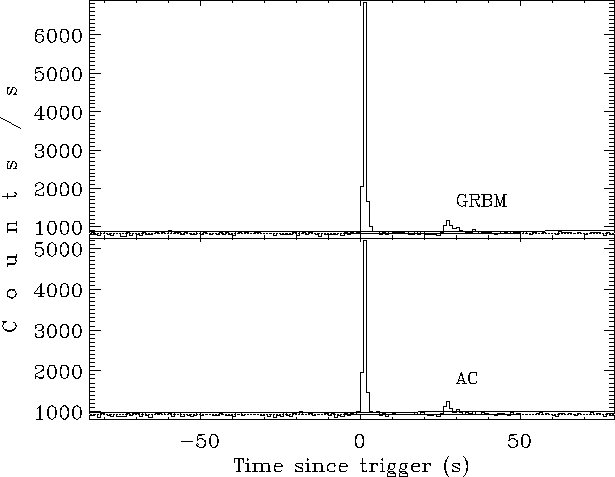
This example refers to GRB010317 (fig. ). The meaning of each line is here explained: the sender (Auto_GRB_monitor@fe.infn.it) and the subject (GRBM/SAX Trigger S/W Alert) are fixed. In the first line there is a total event counter (lkGRB[176]) that numbers the GRB candidate, likewise the trigger number in the case of BATSE; in this case this was the 176th event on-line detected since April 2000. The parameter #LSs gives the number of GRBM units that detected the event: in this case all the units saw it (#LSs: 4); another parameter, called Good HRR, expresses how likely the event is to be a real GRB: this goes from zero (unlikely to be a burst) to six, like in this example, (almost sure burst).

Figure: GRBM unit # 3 light curves of GRB010317: the automatic background fit is shown.

The next two lines report the ``SW Trigger Time'', i.e. the time of the first 1 s bin, in which the SWTCs are triggered, both expressed as OBT (On-Board Time) and UT. Then, whenever the event triggered the on-board logic, there is an optional line reporting the delay between the on-board trigger time and the SW trigger time: in this case, the delay was shorter than 1 s, therefore essentially the same time, if one takes into account that the time resolution of the on-line search is 1 s. The next eight lines are divided into eight columns: from the 1st to the 4th column the data refer to the 40-700 keV energy band of the units #1 to #4; from the 5th to the 8th column the data of the $>$100 keV band of the four units in the same order. In particular, the first two lines ``Nsig(trg)'' and ``Nsig(pfl)'' report in terms of $\sigma$ the counts recorded within the trigger bin and the peak count rate bin, respectively: this example shows that the trigger bin does not coincide with the peak count rate bin. The following line ``Bkg lev.'' reports the background count rate as automatically estimated at the trigger bin. The line tagged ``ChiSq. R.'' indicates the reduced $\chi^2$ come out from the background fit of the surrounding intervals around the burst: this is useful to evaluate how reliable the fit is and, therefore, how good the estimates of the peak count rates and of the total counts are. The next four lines report the peak fluxes (or, more properly, the peak count rates, expressed in counts/s) and the fluences (or total counts) with corresponding errors. Four lines with four columns follow: here the four values in each line refer to the four units, with no distiction between the energy bands: this is because the characteristics reported are computed by taking into account both energy bands of a given unit: the first ``Dur (s)'' clearly reports the time duration expressed in seconds; the duration computation is very simple: it corresponds to the time elapsed from the first to last bin with burst counts; when a short burst is detected, the time duration here reported is 1 or 2 s (the latter case happens when the burst is split between two contiguous 1 s bins). The second line ``Abundance'' yields the numbers of 1 s bins tagged as ``good bins'', i.e. bins with burst counts: when these numbers are lower than their corresponding durations expressed in seconds, like in this example, it means that the burst has a multi-peak profile, since the number of bins exceeding a given threshold is lower than the number of bins included in the burst profile: indeed GRB010317 (fig. ) shows two separate peaks.

Then, the Hardness Ratio line ``H. Ratio'' follows. The ``HR Ratio'', i.e. the Hardness Ratios' Ratio, reports the six values that correspond to the possible ratios between the four HR values in the following order: 1/2, 1/3, 1/4, 2/3, 2/4, 3/4; obviously these are not all independent, as two of them can be derived from the other four. Nevertheless, their values turn to be useful according to an empirical criterium: actually, the greater the number of units with nearly equal HRs among each other, the more likely the transient event to be due to an e.m. radiation plane wave and not to local phenomena, like those induced by particle passages. Strictly speaking, since the burst photons detected by different detector units cross different absorbers, depending on the incoming direction and on the spacecraft payload structure, it turns out that the HRs of the four units are somehow different: anyway, this difference cannot be too big: therefore, the ``Good HRR'' parameter, reported in the very line, expresses the number of HRRs, whose values are within the range $0.8-1.2$ (when $=1$, it means that the two corresponding HRs are equal). The choice for the boundaries, 0.8 and 1.2, resulted from a fine tuning and has come out to be acceptable, after proper tests.

Eventually, the last line reports the weighted average HR with error and must exceed the threshold, set to $0.3$. Usually, GRBs have HR values between 0.5 and 1.0, although in some rare cases 0.3-0.4 can be measured (fig. ); in practice, all the particle events are rejected thanks to this threshold and several solar X-ray flares, too. It seldom happens that solar hard X-ray flares exceed 0.3 by little, and very rarely they may show HR values up to 0.4-0.5. Therefore, as anticipated in the previous chapter, this is perhaps the most important condition to exactly characterize the GRBs among the overall set of transient events usually detected by the GRBM.