The Trigger Conditions

In this section, the description of the late SWTCs is given. Then, the two cases of their application are presented separately: the on- and off-line quests.

The late SWTCs have been conceived in order to improve the background estimate and the selection criteria themselves, so that they could be applied to an on-line quest, without producing an excess of wrong detections, or distributing strongly biased peak flux or fluence estimates of true GRBs.

The most relevant improvement introduced in the background estimate of the ratemeter counts has been achieved by adopting two fitting intervals around the bin to scan, before and after it, and by performing a parabolic fit, instead of the naive average described in eq. . Let $i$th be the scanned bin and $N_b$ and $N_a$ the numbers of bins taken before and after the $i$th bin, respectively ($b$=before, $a$=after); $n_b$ and $n_a$ are defined so that the $(i-n_b)$th bin is the first bin of the $N_b$-bin background fitting interval before the scanned bin, while the $(i+n_a)$th bin is the first bin of the $N_a$-bin background fitting interval after the scanned bin. Let $t(i)$ and $C_u^{(e)}(i)$ be the $i$th time bin and the counts for the $i$th bin, for the energy band $(e)$ and for the detector unit $u$; let ${\mathcal{I}}_t(i)$ be the entire time interval used for the fit and ${\mathcal{I}}(i)$ its corresponding index interval. The background counts $B_u^{(e)}(i)$ are given by the 2nd order polynomial, corresponding to the least square parabolic fit of the two above intervals; to simplify the formulas in the expressions , required for calculating the 2nd order polynomial coefficients, we define $N_{tot}=N_b+N_a$ and we use the notation $c_m(i)$, supposing that $u$ and $e$ are fixed. The two different sets of values used for the on- and off-line quests are reported below and will be discussed more deeply later on in this chapter. In eqq.  some momenta are defined conveniently:

$$\begin{array}{l} N_b = 60, \ N_a = 30, \ n_b = 85, \ n_a = 50 \qq... ...1(i)] \ + \ \bar t_2(i) [\bar t_3(i) - \bar t_2(i)^2]\\ \mbox{}\\ \end{array}$$ (13)

According to the least square method, in order to determine the best fitting polynomial, we resolve the following set of equations :

$$\left\{\begin{array}{l} \displaystyle \frac{{ \partial}}{{\partia... ...b_u^{(e)}(i)\cdot t(k) \, + \, c_u^{(e)}(i)]\Big ]^2 \ = \ 0 \end{array}\right.$$ (14)

The solution to the set of eqq.  gives the following expressions for the coefficients of the parabolic polynomial fitting the background (eqq. ) :

$$\begin{array}{l} a_u^{(e)}(i) = \displaystyle \frac{ m_{21}(i) [ ... ...[ \bar t_3(i)\bar t_1(i) - \bar t_2(i)^2]}{\Delta(i)}\\ \mbox{}\\ \end{array}$$ (15)

Finally, the eq.  gives the background counts $B_u^{(e)}(i)$ :

$$B_u^{(e)}(i) = a_u^{(e)}(i) \cdot [t(i)]^2 \ + \ b_u^{(e)}(i) \cdot t(i) \ + \ c_u^{(e)}(i)$$ (16)

In order to avoid biases of the GRB itself in the background fit, the choice of a proper value for $n_a$, suitable for long duration GRBs in particular, becomes crucial. Actually, a small value for $n_a$ would produce strong biases for all the bursts with time durations greater than $n_a$ s; on the other hand, a very big value for $n_a$ could make the background fit worse, whenever the whole time interval, lasting from the $(i-n_b)$th to the $(i+n_a+N_a)$th bins, would suffer from higher degree polynomial background level variations. Therefore, a proper choice, balancing the undesired effects of these two extreme possibilities, is difficult and must be adapted to the needs of the different quests.

Like in the case of the early SWTCs (see eq. ), we define the net signal $S_u^{(e)}(i) = C_u^{(e)}(i) - B_u^{(e)}(i)$ and the $\sigma_u^{(e)}(i) = \sqrt(B_u^{(e)}(i))$. Let $n_1^{(G)}=3.7$, $n_1^{(A)}=2.5$, $n_2^{(G)}=2.8$, $n_2^{(A)}=2.0$, $n_{min}^{(G)}=1.5$, $n_{min}^{(A)}=1.0$, $n_{tot}^{(G)}=9.0$, $n_{tot}^{(A)}=7.0$, be different threshold parameters, whose meaning will be explained below, in the description of the SWTCs. At this point, all the ingredients required to express the late SWTCs are available: the SWTCs are four, in addition to a further condition on the hardness ratio $HR$ defined below.

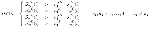
Similarly to the early SWTCs (eq. , , ), the late SWTCs are expressed by the following eqq. , , , :

$$\textrm{SWTC 1} \left\{\begin{array}{l} S_{u_1}^{(G)}(i) \quad > ... ..._2}^{(A)}(i) \end{array}\right. \qquad u_1, u_2=1,\dots,4 \qquad u_1 \not = u_2$$ (17)

$$\textrm{SWTC 2} \left\{\begin{array}{l} S_{u_1}^{(G)}(i) \quad > ... ..._2}^{(A)}(i) \end{array}\right. \qquad u_1, u_2=1,\dots,4 \qquad u_1 \not = u_2$$ (18)

$$\textrm{SWTC 3} \left\{\begin{array}{l} {\mathcal{U}}(i) = \Big\{... ...(A)}(i)}{\sigma_{u}^{(A)}(i)} \quad > \quad n_{tot}^{(A)}\\ \end{array}\right.$$ (19)

$$\textrm{SWTC 4} \left\{\begin{array}{l} S_{u}^{(G)}(k) \quad > \q... ...}\right. \qquad u \in \Big\{1,3\Big\}, \quad \forall k\in \Big\{i-1,i,i+1\Big\}$$ (20)

The SWTC 1 (eq. ) is similar to the early SWTC 1 (eq. ), apart from the different values of the threshold parameters.

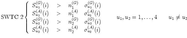
The SWTC 2 (eq. ) is similar to the SWTC 1, with the only difference that the thresholds are no more the same for the two brightest units, but it lowers those for the second brightest one: $n_2^{(G)}=2.8$ in place of $n_1^{(G)}=3.7$ and $n_2^{(A)}=2.0$ in place of $n_1^{(A)}=2.5$.

The SWTC 3 (eq. ) lowers the single unit thresholds and, at the same time, requires that the total sum of the net signals, expressed in $\sigma$, over the set of units matching the lower single unit thresholds, must be greater than a proper threshold, one for each energy band: $n_{tot}^{(G)}$ and $n_{tot}^{(A)}$.

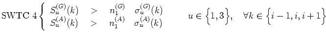
Finally, the SWTC 4 (eq. ) requires that in at least one of the GRBM units 1 and 3, the ones co-aligned with the WFCs (see fig. ), the counts exceed the thresholds in both energy ranges in at least three contiguous bins.