The Sky Grid

Given the above angular resolution, the sky has been split according to a grid consisting of 5292 pixels, obtained by means of the icosahedron-based method for pixelizing the celestial sphere described by [Tegmark, 1996c] ; the angular distance between the centers of two such adjacent pixels amounts to $\sim 3.3\rm ^{\circ}$; thus, the combination of the spacecraft orbit grid with this sky grid allows to study the BeppoSAX sky exposure with an angular resolution of $\sim$3-4$\rm ^{\circ}$.

Figure: Sky Exposure (equatorial coordinates).

Figure: Sky Exposure (galactic coordinates).

For each orbit grid cell ($i, j$) ( $i=1,\ldots,360; j=1,\ldots,8$), a visibility vector $v_{ijk}$ ( $k=1,\ldots,5292$) assumes 1 when the $k$-th sky pixel is surely visible, otherwise 0. Then, a frequency matrix $f_{ij}$ is defined as a function of the orbit grid cells as follows: $f_{ij}$ is the time fraction spent by BeppoSAX within the cell ($i, j$) during the overall time interval considered above; eventually, the sky exposure vector $E_k$ is the product of the following matrices: $E_k = \sum_{i,j} f_{ij} v_{ijk}$. The same procedure has been used for calculating the BeppoSAX local sky exposure, provided that for each observation the celestial sky pixel coordinates are transformed to the local frame of reference. The original 1 s time resolution of the spacecraft ephemerides has been adopted, although a higher time resolution could be used as well, since the arc subtended by the path travelled by BeppoSAX during 1 s amounts to $\sim 3.6\mbox{$^\prime$}$, less than the angular dimensions of the orbit cells; owing to this, a temporal step of $\sim$ 17 s, which is roughly the time needed to cross an orbit cell, could be adopted all the same.

Figure: Sky Exposure as a function of Declination.

Figure: BeppoSAX Local Sky Exposure (GRBM units 1, 2, 3, 4 axes point to $\phi=270\rm ^{\circ}, 0\rm ^{\circ}, 90\rm ^{\circ}, 180\rm ^{\circ}$, respectively, with $\theta=0\rm ^{\circ}$ for all).

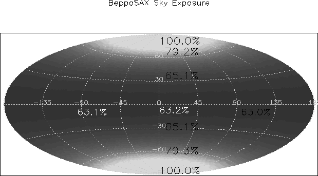
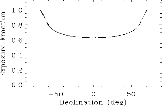
The figure  shows the total sky exposure, expressed in equatorial coordinates; as expected, the equatorial poles are never Earth-blocked, given the low inclination of the BeppoSAX orbit, while the lowest exposure is found at the celestial equator ($\sim 63$%). The functional dependence on declination can be clearly appreciated in fig. , where the small dependence on right ascension has been averaged.

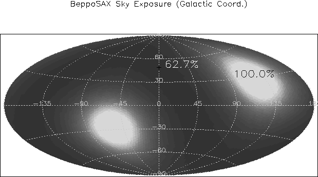
In fig.  the same celestial sky exposure is shown, but now referred to a galactic frame of reference. The maximum exposure regions are obviously found near the equatorial poles.

Figure: BeppoSAX Local Sky Exposure as a function of the local elevation angle $\theta$ for four different $\phi=270\rm ^{\circ}, 0\rm ^{\circ}, 90\rm ^{\circ}, 180\rm ^{\circ}$, corresponding to the normal directions of GRBM units 1, 2, 3, 4, respectively.

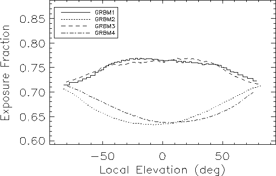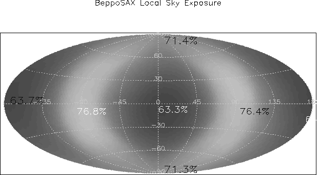
Fig.  shows the BeppoSAX local sky exposure: while the exposure for sky regions close to the axes of GRBM units 1 and 3 is 77-78%, on the other side GRBM units 2 and 4 show a lower exposure amounting to 63-64%. This difference in the local sky exposure is connected with the pointing constraints of the BeppoSAX attitude: in particular, the angle between the Sun and the GRBM unit 2 axis cannot be greater than $\sim 40\rm ^{\circ}$ (see chapter 2). This constraint keeps the unit 2 (and, unit 4 too, since this points to the opposite direction) in the proximity of the ecliptic; therefore, once per orbit the spacecraft units 2 and 4 point to the Earth surface during the BeppoSAX midnight and midday time, respectively, i.e. when the three bodies are aligned, according to the following configurations: BeppoSAX-Earth-Sun and Earth-BeppoSAX-Sun, respectively. This effect is clearly apparent in fig. , where the functional dependence of the local exposure on the elevation $\theta$ above the BeppoSAX equatorial plane is shown, in correspondence of the four GRBM unit axes.