Automatic computation of the total counts

Once a candidate burst triggered one of the SWTCs, an estimate of the total counts is automatically given; the criteria regulating this calculation are illustrated in this section.

Let the $i$th bin be the first bin, for which one of the SWTCs becomes satisfied: from eq.  the background counts $B_u^{(e)}(i)$, used to test the SWTCs, is known.

We conveniently define three intervals: the first of the two intervals used to fit the background, ${\mathcal{B}}(i)$ (${\mathcal{B}}$, i.e. ``Before''), that we call ``pre-burst'', the middle one ${\mathcal{G}}$ (${\mathcal{G}}$, i.e. ``GRB''), containing the burst, therefore, called ``burst'', and the last ${\mathcal{A}}(i)$ (${\mathcal{A}}$, called ``post-burst'',i.e. ``After''):

$$\begin{array}{l} {\mathcal{B}}(i) = \{k\in {\mathbb{N}},\quad (i-... ... = \{k\in {\mathbb{N}},\quad (i+n_a) \leq k \leq (i+n_a+N_a-1)\}\\ \end{array}$$ (22)

In order to evaluate the contribution of the other bins to the total counts of the burst, the same coefficients of the fitting polynomial are used, as expressed in the eq. :

$$B_u^{(e)}(k) = a_u^{(e)}(i) \cdot [t(k)]^2 \, + \, b_u^{(e)}... ... \forall k\in \Big({\mathcal{G}}(i) \cup {\mathcal{A}}(i)\Big)$$ (23)

According to eq. , all the bins belonging to the intervals ${\mathcal{G}}$ and ${\mathcal{A}}$ are taken into account for calculating the total counts.

In order to exclude all the possible bins containing spikes, that could bias the background fit through the coefficients $a_u^{(e)}(i)$, $b_u^{(e)}(i)$ and $c_u^{(e)}(i)$, an iterative fit is performed, once a candidate burst has triggered a SWTC. The iterative fit replaces all the bins, whose counts exceed the background by 3$\sigma$, with the mean of the two contiguous bins: it ends when no more bins are rejected. One cycle of this iterative fit is exactly expressed in the eq. :

$$\tilde{C}_u^{(e)}(k) = \left\{\begin{array}{ll} C_u^{(e)}(k), & \... ...}} > 3.0\\ C_u^{(e)}(k), & \forall k\in {\mathcal{G}}(i)\\ \end{array}\right.$$ (24)

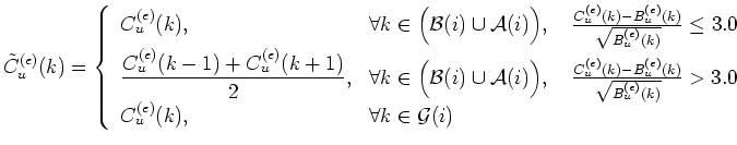
Once the two background fitting intervals ${\mathcal{B}}$ and ${\mathcal{A}}$ have been cleaned from the possible spikes, the net signals $\tilde{S}_u^{(e)}(k)$ for every $k$th bin belonging to the burst and post-burst intervals are defined, according to eq  (the quantities denoted with a tilde are the output of the spike-removing process described just above):

$$\tilde{\sigma}_u^{(e)}(k) = \sqrt{\tilde{B}_u^{(e)}(k)}, \qq... ...ilde{S}_u^{(e)}(k) = \tilde{C}_u^{(e)}(k)-\tilde{B}_u^{(e)}(k)$$ (25)

At this point, the originally triggered SWTC is tested again, since the background coefficients might have changed: if this is no longer satisfied, the candidate burst is discarded; otherwise, each bin with potential counts from the burst is tagged with a flag, distinguishing between the bins with burst counts and the others.

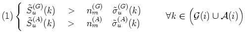
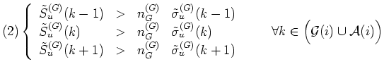
For each single bin, the criteria, that must be matched in order to set the signal flag to positive, are expressed by the two following set of equations:

$$\textrm{(1)} \left\{\begin{array}{l} \tilde{S}_{u}^{(G)}(k) \quad... ...ay}\right. \qquad \forall k\in \Big({\mathcal{G}}(i) \cup {\mathcal{A}}(i)\Big)$$ (26)

$$\textrm{(2)} \left\{\begin{array}{lcll} \tilde{S}_{u}^{(G)}(k-1) ... ...ay}\right. \qquad \forall k\in \Big({\mathcal{G}}(i) \cup {\mathcal{A}}(i)\Big)$$ (27)

When the bin matches at least one among eqq.  and , it is included in the set of ``good'' bins used to estimate the total counts. The values used for the above thresholds are the following: $n_m^{(G)}=2.0$, $n_m^{(A)}=1.5$ and $n_G^{(G)}=2.0$. The meaning of the two sets of criteria is easy and reasonable: in eq.  in both energy bands there must be some signal, while in eq.  enough counts are required in at least three contiguous bins in the GRBM band.

Let ${\mathcal{S}}_u(i)$ be the set of indices of the bins matching at least one of the eqq.  and : this set depends on the trigger bin, that is the $i$th one, and on the unit number $u$.

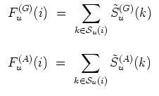
Finally, we have all the elements to define the total counts for both the energy band, $F_u^{(G)}(i)$ for the GRBM band and $F_u^{(A)}(i)$ for the AC band ($F$ means ``fluence'', that should not be confused with that expressed in $\rm erg\ \rm cm2$), for a given detector unit $u$:

$$\begin{array}{l} \displaystyle F_u^{(G)}(i) \ = \ \displaystyle \... ...\displaystyle \sum_{k\in {\mathcal{S}}_u(i)} \tilde{S}_u^{(A)}(k)\\ \end{array}$$ (28)

The automatic estimate of the total counts of a given candidate burst is very important not only because it gives a rough idea of its brightness, but also because its hardness ratio, as computed in the eq. , is fundamental to classify the event itself, since it must fulfil the eq. .

$$\displaystyle HR_u(i) \ = \ \frac{\displaystyle F_u^{(A)}(i)}{\displaystyle F_u^{(G)}(i)}$$ (29)

All these quantities still depend on the $i$th bin, because this is the bin, for which the ratemeters trigger the SWTCs; in other words, the $i$th bin can be identified with the first ``triggering'' bin, and, therefore, with the burst itself. Since the background fit depends on the position of the triggering bin, even the total counts and hardness ratios still keep this little dependence on it, although they express overall properties of the burst.